
The Curious Case of The Red Toyota
Understanding How Conjunction Probability, Base Rates, and Conditional Probability Shape Judgments

The carriage stopped with a jolt outside the Central Bank. Holmes leapt out before the wheels had stilled, his coat flaring like a raven’s wing. Watson, notebook in hand, followed close behind. ‘Another robbery, Holmes?’ I asked. He only gave me a faint smile. “Indeed, Watson. A case of probability,” he replied, his eyes twinkling.
Watson inquired that a gang of robbers stormed the central bank, robbed it at gunpoint, and fled the scene.
The security guard: “They drove off in a car.”
The old lady at the counter: “It was red.”
The kid across the street: “I think it was a Toyota.”
Watson: “Simple enough! We’re looking for a red Toyota, then?”
Holmes (smiling faintly): “Think carefully, Watson. It is always more likely that the robbers fled ‘in a car’ than ‘in a red car,’ and more likely still than ‘in a red Toyota.’ The more details you pile on, the smaller the circle becomes.”
Watson (frowning): “But surely the more details we have, the more certain we become?”
Holmes: “More detailed, yes. More certain, no. Specificity narrows, it does not broaden.”
Conjunction Probability

It’s simple math: a subset can never be larger than its parent set. The chance the robbers fled in a car ≥ the chance they fled in a red car ≥ the chance they fled in a red Toyota.
Every detail makes the story more vivid, but less probable. More generally, the probability of two events occurring together (that is, in conjunction) is always less than or equal to the likelihood of either one occurring by itself. This is representative bias at play. You conflate what is probable with what is plausible. To express it mathematically,
Watson: “But Holmes, if we know it’s a red Toyota, then we can simply search for it. How many can there be?”
Holmes (with a dry chuckle): “In London, Watson? Tens of thousands. The description alone misleads you because you’ve neglected the base rate. If there are sixty thousand red Toyotas in the city, then our clue is far weaker than it appears.”
Base Rate
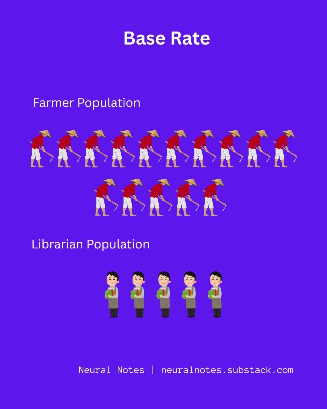
The sample sizes tend to determine the probability of events. Imagine this: you are told that Steve is shy and wears spectacles. Who is Steve more likely to be, a librarian or a farmer? Intuitively, you might answer that Steve is a librarian. But in reality, Steve is much more likely to be a farmer. The reason is that you are ignoring the base rate.
If you look at the demographics, the population of farmers, in general, is greater than the population of librarians. Assume that there are five farmers for every one librarian. We observe that 30% of the farmer’s population wears spectacles, and about 50% (a lot higher percentile, mind you) among the librarians.
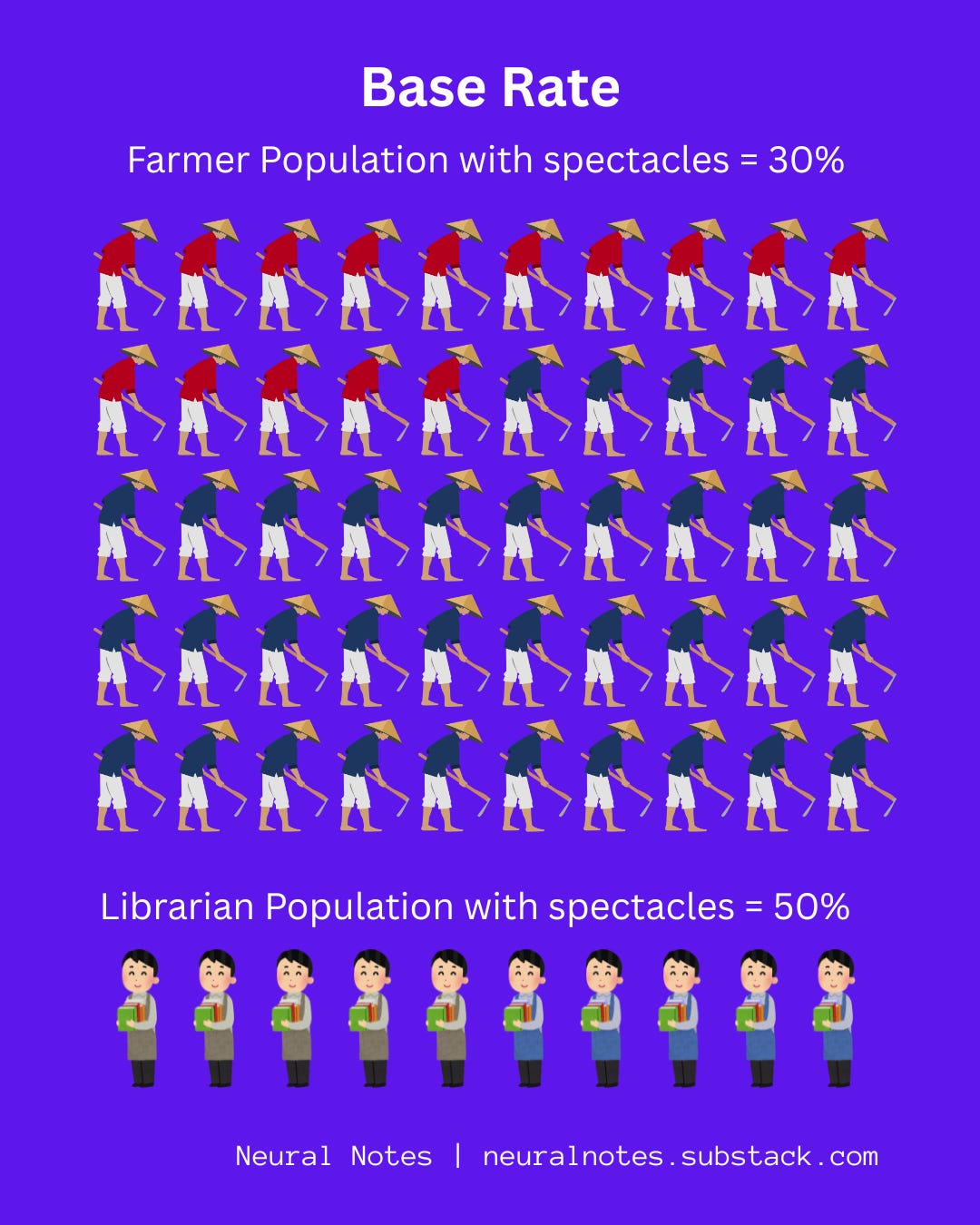
It sounds like spectacles are more common among librarians, but when you count the actual numbers, things flip.
Notice how the number of farmers with spectacles is a lot higher purely because there are just more farmers than there are librarians. In this case, we have 15 farmers (30%) and 5 librarians (50%) matching the description. So, if you meet a shy man with spectacles, there is a 75% chance he is a farmer and only a 25% chance he is a librarian. The description may feel as if it points toward a librarian, but the larger population of farmers makes it far more likely that Steve is one of them. Therefore, the description is much more likely to match with a farmer than a librarian, counter to what you initially assumed! This mistake, where we ignore how common something is in the background and focus only on the description, is called the base rate fallacy or base rate neglect.
Always check how big the buckets are before you guess which bucket something belongs to.
From the earlier example on robbery, suppose the city had 60,000 red Toyotas. Then the detail “red Toyota” tells you almost nothing because the base rate is high. But if there are only 600 in the whole city, suddenly the clue is powerful to catch the robbers.
Watson: “At least one thing is clear: if there’s been a robbery, the gang probably escaped in a car. Most robbers don’t run off on foot.”
Holmes (nodding): “Quite so. But turn the question around, Watson. If you see a red Toyota on the street, what are the chances it was the getaway car? That, I’m afraid, is vanishingly small. The first question asks what robbers tend to do. The second asks what Toyotas tend to do. A very different matter.”
Watson (sighing): “So one is about criminals’ habits… and the other is about cars’ habits.”
Holmes (smiling faintly): “Exactly, my dear Watson.”
Conditional Probability
Events can either be independent or dependent.
An event is independent if its outcome is not influenced by what happened before. For instance, each toss of a fair coin is independent. Whether you just got heads five times in a row has no effect on what comes next.
An event is dependent if the outcome does change based on what happened before. For example, if you draw a card from a deck without replacement, the probability shifts. At first, the chance of drawing a spade is 13 out of 52. But if you already drew one card and didn’t put it back, now the chance is calculated out of 51. The second draw depends on the first.
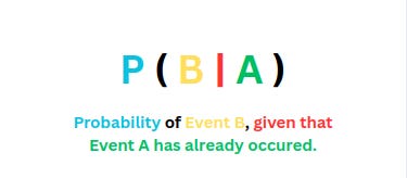
Therefore, we have unconditional probabilities and conditional probabilities. Conditional probabilities are the chances of an event B happening, given that event A has already occurred. Returning to the earlier card example, what is the probability of drawing a spade next given that the first draw was a club?
Let’s calculate. Below is the picture of a deck of cards laid out on a table. A standard deck of cards typically consists of 52 cards divided into four suits: hearts, diamonds, clubs, and spades, with each suit containing 13 ranks.
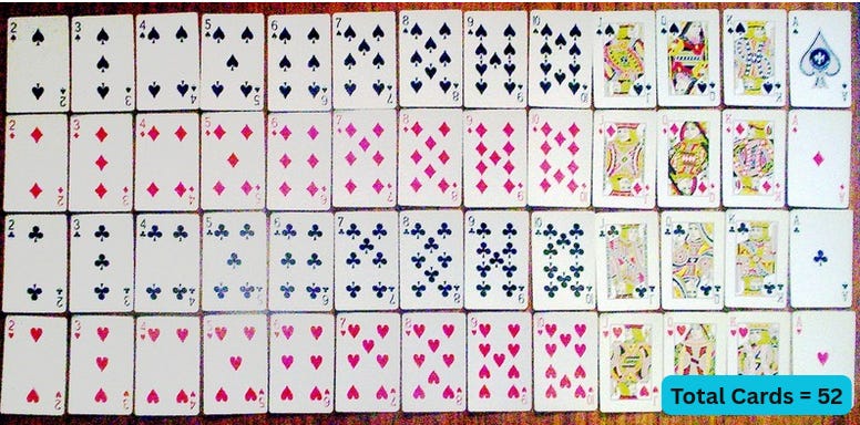
Event A: You drew a 4 of clubs (without replacement). Now there are 51 cards left.
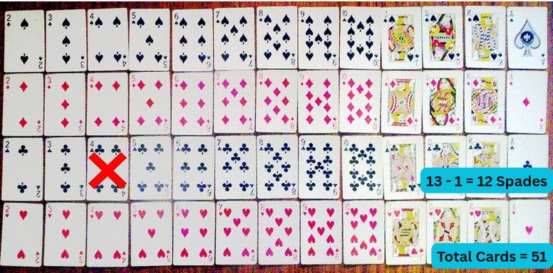
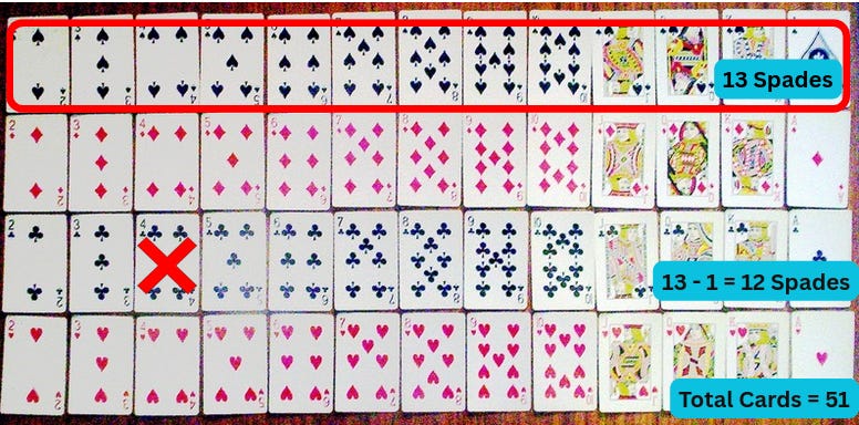
Event B: Drawing a spade. Looking at the image, you can see all 13 spades are still there.
Conditional Probability: What is the probability of Event B, given the information that Event A has already occurred?
In other words, what is the probability of drawing a spade, given that a club has already been drawn. Mathematically, it is expressed as:
Since the deck has only 51 cards and all 13 spades remain, the conditional probability of drawing a spade given that the first draw was a club is:
There is a 25.5% chance that you will draw a spade out of the deck, given that you already drew a club.
Going back to the crime scene, Holmes explains to Watson, “what’s the chance the robbers used a car to get away? Pretty high, since most robbers don’t sprint off on foot.”
“But flip the question, Watson,” says Holmes, “Given that you spot a red Toyota, what’s the chance it was the getaway car? Now the base rate kicks in. If the city has 60,000 red Toyotas and only one of them was involved in the robbery, the chance that the one you happen to see is the getaway car is 1 in 60,000, which is vanishingly small.”
That’s the key difference: P ( Car | Robbery ) (most robbers use cars) feels very different from P ( Robbery | Red Toyota ) (most red Toyotas are not used in robberies).
“Watson,” Holmes said quietly, “never forget: the world is full of stories, but it’s numbers that tell the truth.”
If you're interested in the "Science of Deduction," read my newsletter on Bayes' Theorem:
